IPython的魔法符号－Magics

openthings@163.com

最新的Jupyter Notebook可以混合执行Shell、Python以及Ruby、R等代码！

这一功能将解释型语言的特点发挥到了极致，从而打破了传统语言"运行时"的边界。

IPython是一个非常好用Python控制台，极大地扩展了Python的能力。

因为它不仅是一种语言的运行环境，而且是一个高效率的分析工具。

*

之前任何语言和IDE都是相互独立的，导致工作时需要在不同的系统间切换和拷贝／粘贴数据。 * Magic操作符可以在HTML页面中输入shell脚本以及Ruby等其它语言并混合执行，极大地提升了传统的“控制台”的生产效率。 * Magics是一个单行的标签式“命令行”系统，指示后续的代码将如何、以及被何种解释器去处理。 * Magisc与传统的shell脚本几乎没有什么区别，但是可以将多种指令混合在一起。

Magics 主要有两种语法:

• Line magics: 以 % 字符开始，该行后面都为指令代码，参数用空格隔开，不需要加引号。
• Cell magics: 使用两个百分号 (%%)开始, 后面的整个单元（Cell）都是指令代码。 注意，%%魔法操作符只在Cell的第一行使用，而且不能嵌套、重复（一个Cell只有一个）。极个别的情况，可以堆叠，但是只用于个别情况。

输入 [%lsmagic] 可以获得Magic操作符的列表。

如下所示（在Jupyter Notebook环境下，按[shift+enter]可以运行。）：

In [ ]:

%lsmagic

**

缺省情况下，Automagic开关打开，不需要输入%符号，将会自动识别。** | 注意，这有可能与其它的操作引起冲突，需要注意避免。如果有混淆情况，加上%符号即可。

下面显示运行一段代码所消耗的时间。

In [26]:

time print("hi")

hi
CPU times: user 0 ns, sys: 0 ns, total: 0 ns
Wall time: 47.9 µs

In [27]:

%time

CPU times: user 0 ns, sys: 0 ns, total: 0 ns
Wall time: 4.77 µs

执行Shell脚本。

In [9]:

ls -l -h

总用量 340K
-rw-rw-r-- 1 supermap supermap 266K  4月 29 09:29 jupyter_magics.ipynb
-rw-rw-r-- 1 supermap supermap  58K  4月 27 12:38 pandas_quickstart.ipynb
-rw-rw-r-- 1 supermap supermap  12K  4月 27 12:28 pystart_databasic.ipynb

In [10]:

!ls -l -h

总用量 340K
-rw-rw-r-- 1 supermap supermap 266K  4月 29 09:29 jupyter_magics.ipynb
-rw-rw-r-- 1 supermap supermap  58K  4月 27 12:38 pandas_quickstart.ipynb
-rw-rw-r-- 1 supermap supermap  12K  4月 27 12:28 pystart_databasic.ipynb

In [16]:

files = !ls -l -h
files

Out[16]:

['总用量 348K',
 '-rw-rw-r-- 1 supermap supermap 276K  4月 29 09:31 jupyter_magics.ipynb',
 '-rw-rw-r-- 1 supermap supermap  58K  4月 27 12:38 pandas_quickstart.ipynb',
 '-rw-rw-r-- 1 supermap supermap  12K  4月 27 12:28 pystart_databasic.ipynb']

执行多行shell脚本。

In [25]:

%%!
ls -l
pwd
who

Out[25]:

['总用量 344',
 '-rw-rw-r-- 1 supermap supermap 274868  4月 29 09:33 jupyter_magics.ipynb',
 '-rw-rw-r-- 1 supermap supermap  59280  4月 27 12:38 pandas_quickstart.ipynb',
 '-rw-rw-r-- 1 supermap supermap  11528  4月 27 12:28 pystart_databasic.ipynb',
 '/home/supermap/GISpark/git_notebook/pystart',
 'supermap :0           2016-04-28 20:39 (:0)',
 'supermap pts/0        2016-04-28 21:50 (:0)',
 'supermap pts/6        2016-04-28 22:22 (:0)']

下面开始体验一下魔法操作符的威力。

载入matplotlib和numpy，后面的数值计算和绘图将会使用。

---

%timeit 魔法，计量代码的执行时间, 适用于单行和cell:

In [50]:

%timeit np.linalg.eigvals(np.random.rand(100,100))

The slowest run took 8.96 times longer than the fastest. This could mean that an intermediate result is being cached.
100 loops, best of 3: 5.82 ms per loop

In [4]:

%%timeit a = np.random.rand(100, 100)
np.linalg.eigvals(a)

100 loops, best of 3: 6.07 ms per loop

%%capture 魔法，用于捕获stdout/err, 可以直接显示，也可以存到变量里备用:

In [4]:

%%capture capt
from __future__ import print_function
import sys
print('Hello stdout')
print('and stderr', file=sys.stderr)

In [5]:

capt.stdout, capt.stderr

Out[5]:

('Hello stdout\n', 'and stderr\n')

In [53]:

capt.show()

Hello stdout

and stderr

%%writefile 魔法，将后续的语句写入文件中:

In [8]:

%%writefile foo.py
print('Hello world')

Writing foo.py

In [9]:

%run foo

Hello world

Magics 运行其它的解释器。

---

执行时从stdin取得输入，就像你自己在键入一样。

直接在%%script 行后传入指令即可使用。

后续的cell中的内容将按照指示符运行，子进程的信息通过stdout/err捕获和显示。

In [1]:

%%script python
import sys
print('hello from Python %s' % sys.version)

hello from Python 3.5.1 |Anaconda 4.0.0 (64-bit)| (default, Dec  7 2015, 11:16:01)
[GCC 4.4.7 20120313 (Red Hat 4.4.7-1)]

In [2]:

%%script python3
import sys
print('hello from Python: %s' % sys.version)

hello from Python: 3.5.1 |Anaconda 4.0.0 (64-bit)| (default, Dec  7 2015, 11:16:01)
[GCC 4.4.7 20120313 (Red Hat 4.4.7-1)]

IPython对通用的解释器创建了别名，可以直接使用, 譬如：bash, ruby, perl,

etc. | **等价于这个操作符： %%script <name> **

In [3]:

%%ruby
puts "Hello from Ruby #{RUBY_VERSION}"

Hello from Ruby 2.1.5

In [4]:

%%bash
echo "hello from $BASH"

hello from /bin/bash

写一个脚本文件，名为 lnum.py, 然后执行：

In [6]:

%%writefile ./lnum.py
print('my first line.')
print("my second line.")
print("Finished.")

Writing ./lnum.py

In [33]:

%%script python ./lnum.py
#

my first line.
my second line.
Finished.

可以直接从子进程中捕获stdout/err到Python变量中, 替代直接进入stdout/err。

In [14]:

%%bash
echo "hi, stdout"
echo "hello, stderr" >&2

hi, stdout

hello, stderr

In [15]:

%%bash --out output --err error
echo "hi, stdout"
echo "hello, stderr" >&2

可以直接访问变量名了。

In [17]:

print(error)
print(output)

hello, stderr

hi, stdout

只需添加 ``–bg`` ，即可让脚本在后台运行。

在此情况下, 输出将被丢弃，除非使用 --out/err 捕获输出。

In [34]:

%%ruby --bg --out ruby_lines
for n in 1...10
    sleep 1
    puts "line #{n}"
    STDOUT.flush
end

Starting job # 2 in a separate thread.

当后台线程保存输出时，有一个stdout/err pipes, 而不是输出的文本形式。

In [35]:

ruby_lines

Out[35]:

<_io.BufferedReader name=52>

In [36]:

print(ruby_lines.read())

b'line 1\nline 2\nline 3\nline 4\nline 5\nline 6\nline 7\nline 8\nline 9\n'

Cython Magic 函数扩展

IPtyhon 包含 cythonmagic extension，提供了几个与Cython代码工作的魔法函数。使用 %load_ext 载入，如下:

In [37]:

%load_ext cythonmagic

/home/supermap/anaconda3/envs/GISpark/lib/python3.5/site-packages/IPython/extensions/cythonmagic.py:21: UserWarning: The Cython magic has been moved to the Cython package
  warnings.warn("""The Cython magic has been moved to the Cython package""")

** %%cython_pyximport** magic函数允许你在Cell中使用任意的Cython代码。Cython代码被写入.pyx 文件，保存在当前工作目录，然后使用pyximport 引用进来。需要指定一个模块的名称，所有的符号将被自动import。

In [38]:

%%cython_pyximport foo
def f(x):
    return 4.0*x

ERROR: Cell magic `%%cython_pyximport` not found.

In [6]:

f(10)

Out[6]:

40.0

%cython magic类似于 %%cython_pyximport magic, 但不需要指定一个模块名称. %%cython magic 使用 ~/.cython/magic目录中的临时文件来管理模块，所有符号会被自动引用。

下面是一个使用Cython的例子，Black-Scholes options pricing algorithm:

In [39]:

%%cython
cimport cython
from libc.math cimport exp, sqrt, pow, log, erf

@cython.cdivision(True)
cdef double std_norm_cdf(double x) nogil:
    return 0.5*(1+erf(x/sqrt(2.0)))

@cython.cdivision(True)
def black_scholes(double s, double k, double t, double v,
                 double rf, double div, double cp):
    """Price an option using the Black-Scholes model.

    s : initial stock price
    k : strike price
    t : expiration time
    v : volatility
    rf : risk-free rate
    div : dividend
    cp : +1/-1 for call/put
    """
    cdef double d1, d2, optprice
    with nogil:
        d1 = (log(s/k)+(rf-div+0.5*pow(v,2))*t)/(v*sqrt(t))
        d2 = d1 - v*sqrt(t)
        optprice = cp*s*exp(-div*t)*std_norm_cdf(cp*d1) - \
            cp*k*exp(-rf*t)*std_norm_cdf(cp*d2)
    return optprice

ERROR: Cell magic `%%cython` not found.

In [40]:

black_scholes(100.0, 100.0, 1.0, 0.3, 0.03, 0.0, -1)

---------------------------------------------------------------------------
NameError                                 Traceback (most recent call last)
<ipython-input-40-ae31cbfa5fba> in <module>()
----> 1 black_scholes(100.0, 100.0, 1.0, 0.3, 0.03, 0.0, -1)

NameError: name 'black_scholes' is not defined

测量一下运行时间。

In [45]:

#%timeit black_scholes(100.0, 100.0, 1.0, 0.3, 0.03, 0.0, -1)

Cython 允许使用额外的库与你的扩展进行链接，采用 -l 选项 (或者 --lib)。 注意，该选项可以使用多次，libraries, such as -lm -llib2 --lib lib3. 这里是使用 system math library的例子:

In [10]:

%%cython -lm
from libc.math cimport sin
print 'sin(1)=', sin(1)

sin(1)= 0.841470984808

同样，可以使用 -I/--include 来指定包含头文件的目录, 以及使用 -c/--compile-args 编译选项，以及 extra_compile_args of the distutils Extension class. 请参考 the Cython docs on C library usage 获得更详细的说明。

Rmagic 函数扩展

IPython 通过 rmagic

扩展来调用R模块，是通过rpy2来实现的(安装：conda install rpy2)。 | rpy2的文档：http://rpy2.readthedocs.io/en/version_2.7.x/ #### 首先使用 %load_ext 载入该模块: 注意：新的rpy2已改动，不能运行。参考：http://rpy2.readthedocs.io/en/version_2.7.x/interactive.html?highlight=rmagic

In [58]:

%reload_ext rmagic

/home/supermap/anaconda3/envs/GISpark/lib/python3.5/site-packages/IPython/extensions/rmagic.py:11: UserWarning: The rmagic extension in IPython has moved to `rpy2.ipython`, please see `rpy2` documentation.
  warnings.warn("The rmagic extension in IPython has moved to "

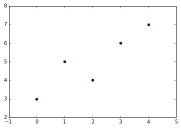
典型的用法是使用R来计算numpy的Array的统计指标。我们试一下简单线性模型，输出scatterplot。

In [62]:

%matplotlib inline
import numpy as np
import matplotlib.pyplot as plt

In [63]:

X = np.array([0,1,2,3,4])
Y = np.array([3,5,4,6,7])
plt.scatter(X, Y)

Out[63]:

<matplotlib.collections.PathCollection at 0x7f9760cdd208>

首先把变量赋给 R, 拟合模型并返回结果。 %Rpush 拷贝 rpy2中的变量. %R 对 rpy2 中的字符串求值，然后返回结果。在这里是线性模型的协方差－coefficients。

In [64]:

%Rpush X Y
%R lm(Y~X)$coef

ERROR: Line magic function `%Rpush` not found.
ERROR: Line magic function `%R` not found.

%R可以返回多个值。

In [65]:

%R resid(lm(Y~X)); coef(lm(X~Y))

ERROR: Line magic function `%R` not found.

可以将 %R 结果传回 python objects. 返回值是一个“；”隔开的多行表达式，coef(lm(X~Y)).

拉取R的其它变量, 采用 %Rpull 和 %Rget. 在 R code 执行后，在 rpy2

namespace 有变量需要获取。 | 主要区别是： (%Rget)返回值, 而(%Rpull)从 self.shell.user_ns 拉取。想象一下，我们计算得到变量 “a” 在rpy2’s namespace. 使用 %R magic, 我们得到结果并存储到 b。可以从 user_ns 使用 %Rpull得到。返回的是同一个数据。

In [6]:

b = %R a=resid(lm(Y~X))
%Rpull a
print(a)
assert id(b.data) == id(a.data)
%R -o a

[-0.2  0.9 -1.   0.1  0.2]

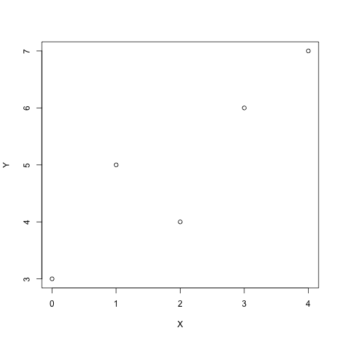
R的控制台stdout()被ipython捕获。

In [7]:

from __future__ import print_function
v1 = %R plot(X,Y); print(summary(lm(Y~X))); vv=mean(X)*mean(Y)
print('v1 is:', v1)
v2 = %R mean(X)*mean(Y)
print('v2 is:', v2)

Call:
lm(formula = Y ~ X)

Residuals:
   1    2    3    4    5
-0.2  0.9 -1.0  0.1  0.2

Coefficients:
            Estimate Std. Error t value Pr(>|t|)
(Intercept)   3.2000     0.6164   5.191   0.0139 *
X             0.9000     0.2517   3.576   0.0374 *
---
Signif. codes:  0 ‘***’ 0.001 ‘**’ 0.01 ‘*’ 0.05 ‘.’ 0.1 ‘ ’ 1

Residual standard error: 0.7958 on 3 degrees of freedom
Multiple R-squared:   0.81, Adjusted R-squared:  0.7467
F-statistic: 12.79 on 1 and 3 DF,  p-value: 0.03739

v1 is: [ 10.]
v2 is: [ 10.]

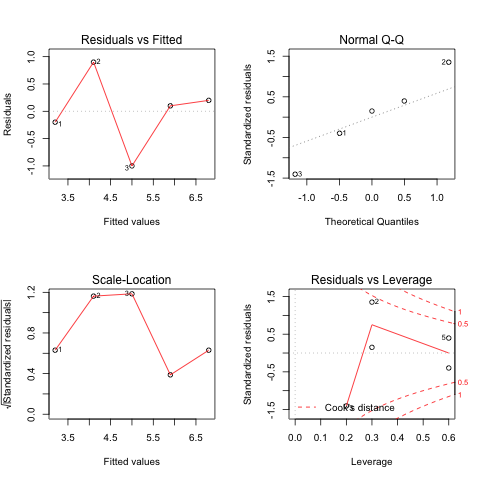
我们希望用R在cell级别。而且numpy最好不要转换，参考R: rnumpy ( http://bitbucket.org/njs/rnumpy/wiki/API ) 。

In [8]:

%%R -i X,Y -o XYcoef
XYlm = lm(Y~X)
XYcoef = coef(XYlm)
print(summary(XYlm))
par(mfrow=c(2,2))
plot(XYlm)

Call:
lm(formula = Y ~ X)

Residuals:
   1    2    3    4    5
-0.2  0.9 -1.0  0.1  0.2

Coefficients:
            Estimate Std. Error t value Pr(>|t|)
(Intercept)   3.2000     0.6164   5.191   0.0139 *
X             0.9000     0.2517   3.576   0.0374 *
---
Signif. codes:  0 ‘***’ 0.001 ‘**’ 0.01 ‘*’ 0.05 ‘.’ 0.1 ‘ ’ 1

Residual standard error: 0.7958 on 3 degrees of freedom
Multiple R-squared:   0.81, Adjusted R-squared:  0.7467
F-statistic: 12.79 on 1 and 3 DF,  p-value: 0.03739

octavemagic: Octave inside IPython

``octavemagic`` 提供与Octave交互的能力。依赖 oct2py 和

h5py 软件包。 | 载入扩展包:

%load_ext octavemagic

载入这个扩展包，启用了三个magic functions: %octave,

%octave_push, 和 %octave_pull。 | 第一个执行一行或多行Octave, 后面两个执行 Octave 和 Python 的变量交换。

In [110]:

x = %octave [1 2; 3 4];
x

Out[110]:

array([[ 1.,  2.],
       [ 3.,  4.]])

In [111]:

a = [1, 2, 3]

%octave_push a
%octave a = a * 2;
%octave_pull a
a

Out[111]:

array([[2, 4, 6]])

``%%octave`` : 多行 Octave 被执行。但与单行不同, 没有值被返回, 我们使用-i 和 -o 指定输入和输出变量。

In [116]:

%%octave -i x -o y
y = x + 3;

In [117]:

y

Out[117]:

array([[ 4.,  5.],
       [ 6.,  7.]])

Plot输出自动被捕获和显示，使用 -f 参数选择输出的格式 (目前支持 png 和 svg)。

In [118]:

%%octave -f svg

p = [12 -2.5 -8 -0.1 8];
x = 0:0.01:1;

polyout(p, 'x')
plot(x, polyval(p, x));

12*x^4 - 2.5*x^3 - 8*x^2 - 0.1*x^1 + 8

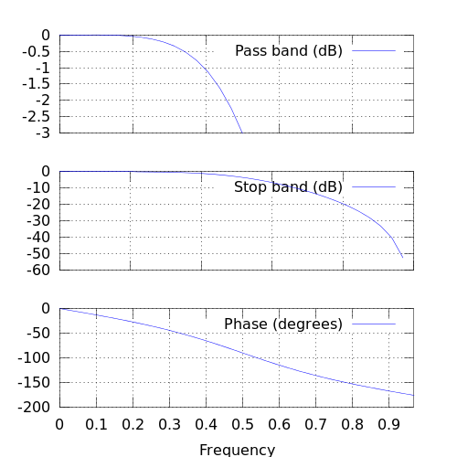
使用 -s 参数调整大小:

In [119]:

%%octave -s 500,500

# butterworth filter, order 2, cutoff pi/2 radians
b = [0.292893218813452  0.585786437626905  0.292893218813452];
a = [1  0  0.171572875253810];
freqz(b, a, 32);

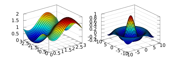
In [120]:

%%octave -s 600,200 -f png

subplot(121);
[x, y] = meshgrid(0:0.1:3);
r = sin(x - 0.5).^2 + cos(y - 0.5).^2;
surf(x, y, r);

subplot(122);
sombrero()